Why Keeping Your Learning Rate Small is Crucial
When training a neural network, every parameter choice significantly impacts the model’s performance. One of the most crucial parameters is the rate at which your model learns. This seemingly small detail can determine whether your model finds the optimal solution or fails to converge at all.
In this post, we’ll dive deep into the importance of the rate at which adjustments are made, how it affects your model’s training process, and why a conservative approach can lead to better outcomes. We’ll also explore practical tips on setting the right pace for learning, common pitfalls to avoid, and how to monitor your model’s progress to ensure optimal performance.
Understanding the Learning Rate
The rate of learning dictates how quickly or slowly your model updates its weights during training. A slow pace allows the model to make incremental changes, carefully adjusting the weights in response to the gradient of the loss function. Conversely, a faster pace might cause the model to overshoot the optimal weights, potentially missing the global minima—the point where the loss function is at its lowest.
But why is this such a crucial factor in training neural networks? To answer this, let’s break down what happens during the training process.
The Training Process and the Role of Learning Adjustments
Training a neural network involves multiple iterations (or epochs) over the dataset. During each iteration, the model makes predictions, calculates the error (or loss), and updates its weights to minimize this error. This update process is guided by the gradient descent algorithm, where the adjustment pace acts as the step size—dictating how big or small the steps are that the model takes toward minimizing the loss.
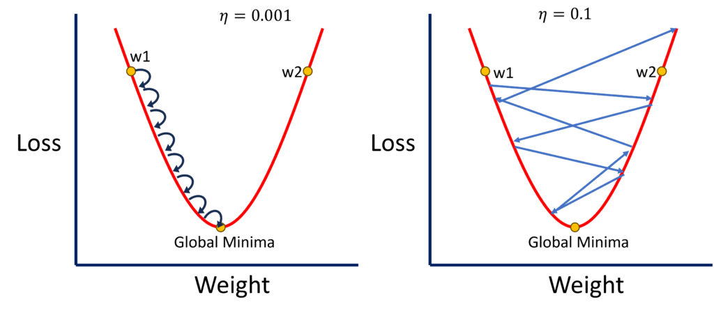
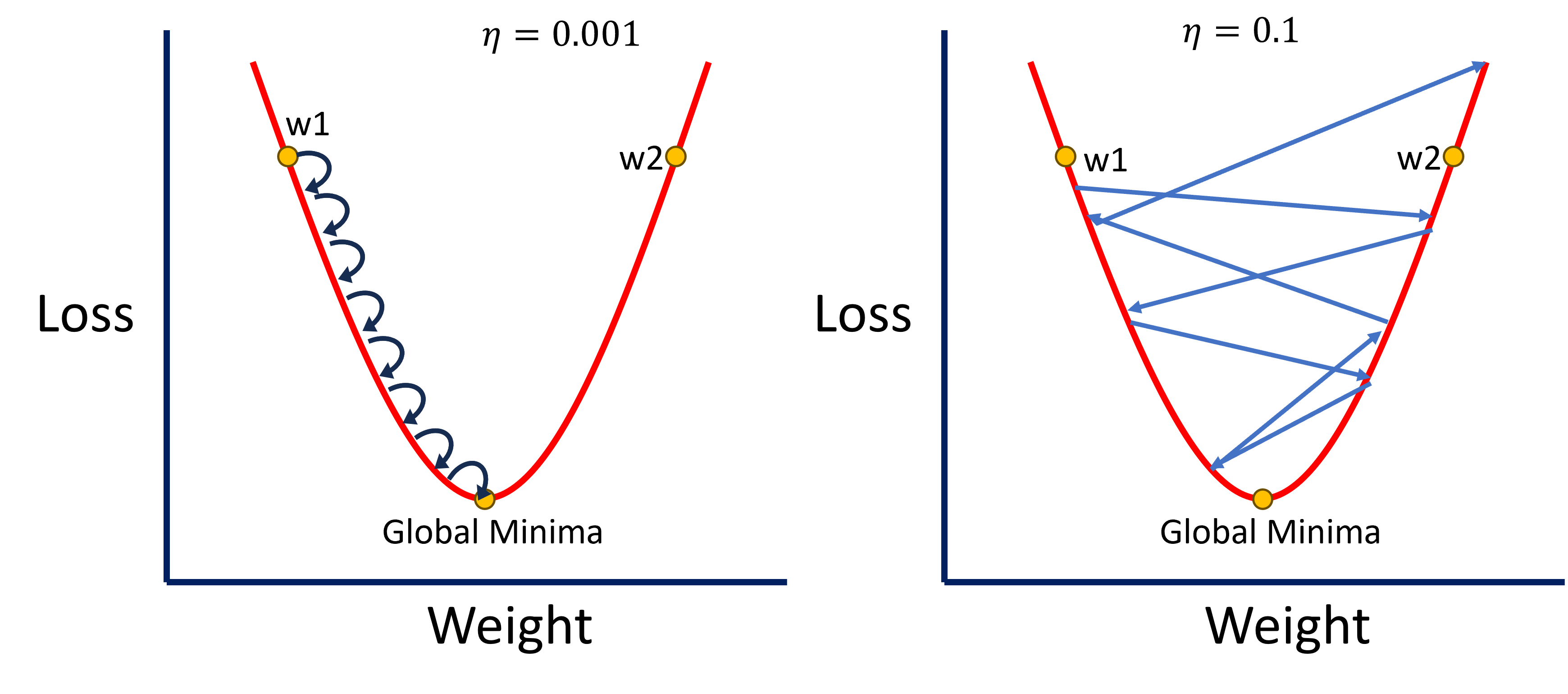
- Small Rate: When the pace is slow, the model makes tiny adjustments to the weights. This cautious approach allows the model to carefully navigate the error landscape, steadily moving toward the global minima without overshooting.
- Large Rate: On the other hand, a rapid pace can cause the model to take too large steps. While this might speed up the training process initially, it can also cause the model to oscillate around the optimal solution or even diverge from it entirely.
Now that we understand the basic concept, let’s explore why keeping the pace conservative can be beneficial.
1. Convergence to Global Minima
When the learning adjustments are small, it enables the model’s weights to converge more effectively to the global minima of the loss function. The global minima represent the most optimized solution where the error between the predicted and actual outputs is minimized. A slow and steady approach ensures that the model makes fine-tuned adjustments, gradually descending the gradient to find the lowest point.
Example: Imagine you’re navigating a steep mountain in dense fog. If you take small, careful steps, you’re more likely to reach the bottom safely, avoiding sharp drops or obstacles. Similarly, a cautious adjustment rate allows the model to make careful changes, ensuring it reaches the global minima without overshooting.
In contrast, if the adjustment rate is too large, the model may skip over the global minima, oscillating around the optimal solution without ever settling down. This lack of convergence can lead to a model that underperforms, as it never reaches the ideal configuration of weights that would yield the highest accuracy.
Consider the weight update formula:
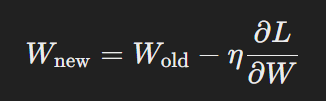
where η is the learning adjustment rate, L is the loss, and W represents the weights. When η is small (e.g., 0.001), the changes to the weights are minimal, allowing for a more precise approach to finding the global minima. However, with a larger η (e.g., 0.1), the weight updates are more substantial, increasing the risk of overshooting the optimal point.
2. Avoiding Divergence
A rapid pace not only risks missing the global minima but can also cause the model to diverge entirely from a viable solution. When the rate is excessively high, the updates to the weights are too aggressive, potentially pushing the model in the wrong direction and causing it to exit the gradient descent prematurely.
Understanding Divergence: Divergence occurs when the model’s weights move so far from the optimal path that the loss increases rather than decreases. This can result in a model that performs worse over time, as the learning process becomes unstable. To avoid this pitfall, maintaining a small and steady adjustment rate ensures that the model remains on track, steadily decreasing the loss and improving accuracy.
Visualizing Divergence
Imagine a scenario where you’re trying to navigate a labyrinth. If you rush through it (analogous to having a large rate), you’re more likely to take wrong turns and end up farther from the exit. Conversely, if you proceed slowly and cautiously (small rate), you’re more likely to find the correct path, even if it takes longer.
In practical terms, a model with a rapid pace might start with a lower loss but could quickly spiral out of control, leading to poor performance. This is why it’s often recommended to start with a slow rate and gradually increase it, allowing the model to adjust smoothly.
3. Achieving Stability in Training
Training stability is another crucial factor influenced by the rate of learning. With a small rate, the model’s training process is more stable, as the weight updates are gradual and less likely to cause sudden, erratic changes in performance. This stability is particularly important in complex models, where slight adjustments can have a significant impact on the outcome.
Example: In a marathon, a steady pace often yields better results than sprinting intermittently and exhausting yourself. Similarly, a small and consistent adjustment pace ensures that the model makes steady progress, improving its performance over time.
Stable training allows the model to learn more effectively, building on its progress with each epoch. In contrast, a rapid rate can lead to instability, where the model’s performance fluctuates wildly, making it difficult to achieve consistent improvements.
4. Enhancing Generalization
One often overlooked benefit of a small adjustment rate is its positive impact on the model’s generalization capabilities. Generalization refers to the model’s ability to perform well on unseen data—an essential aspect of creating robust AI models.
How It Works: When the rate is small, the model’s weight adjustments are more refined, reducing the likelihood of overfitting. Overfitting occurs when a model becomes too specialized in the training data, performing exceptionally well on it but poorly on new, unseen data. By keeping the adjustment rate low, you allow the model to generalize better, as it’s less likely to latch onto noise or irrelevant patterns in the training data.
5. Practical Considerations for Choosing the Learning Rate
While a conservative adjustment pace offers several advantages, it’s important to strike the right balance. If the rate is too small, training can become unbearably slow, requiring more epochs to achieve convergence. A common practice is to start with a moderate rate and adjust it based on the model’s performance during training. Techniques such as learning rate schedules, where the rate is gradually reduced over time, can also be effective in finding the optimal balance.
Learning Rate Schedules: These are methods to adjust the learning rate during training dynamically. Common strategies include:
- Step Decay: The rate is reduced by a factor after a fixed number of epochs.
- Exponential Decay: The rate decreases exponentially as the training progresses.
- Cosine Annealing: The rate follows a cosine function, decreasing over time but occasionally increasing in a wave-like pattern.
Each of these methods helps fine-tune the learning process, ensuring that the model continues to improve without the risks associated with a constant pace.
6. Using Learning Rate Finders
One effective technique to identify the optimal learning rate is using a learning rate finder. This approach involves training the model on a small subset of data, starting with a very low rate and gradually increasing it. By plotting the loss against the rate, you can identify the point where the loss starts decreasing significantly and where it starts to increase again. The optimal rate is typically just before the loss begins to rise.
Implementation: Many popular deep learning libraries, such as PyTorch and TensorFlow, include built-in functions for learning rate finders. This method provides a more empirical approach to setting the rate, rather than relying on guesswork or fixed values.
7. Combining Learning Rate with Momentum
In some cases, combining a small learning rate with momentum can lead to even better results. Momentum helps the model to continue moving in the right direction by adding a fraction of the previous update to the current one. This can help the model to navigate the error landscape more efficiently, especially when the loss surface is complex and full of local minima.
Formula:

where ΔWprev represents the previous weight update, and momentum is typically set between 0.5 and 0.9.
By combining a small learning rate with momentum, you can achieve smoother convergence, as the momentum helps the model to build up speed in the right direction while avoiding the pitfalls of a large rate.
To Learn more Click Here
8. Monitoring and Adjusting the Learning Rate
Setting the initial learning rate is just the beginning. Throughout the training process, it’s essential to monitor the model’s performance and adjust the rate as needed. This can be done through various techniques:
- Early Stopping: Stop training when the model’s performance on a validation set starts to deteriorate. This prevents overfitting and indicates that the learning rate might be too high.
- Learning Rate Warm-up: Start with a smaller rate for the first few epochs and gradually increase it. This helps stabilize the initial training phase, especially in models with high variance.
- Cyclic Learning Rates: Alternate between high and low rates during training. This method can help the model escape local minima and explore different parts of the error landscape.
Conclusion: Why a Small Learning Rate Matters
In summary, keeping your learning rate small can have a profound impact on your model’s success. It ensures that the weights converge to the global minima, avoids the risks of divergence, promotes stable, effective training, enhances generalization, and allows for fine-tuning through various techniques. By carefully choosing and adjusting the learning rate, you can optimize your neural network for better accuracy and performance.
Support Our Mission
At DataSwag, we are committed to making data science and machine learning accessible to everyone. To support our mission and continue providing valuable content, check out our exclusive merchandise on DataSwag. Your purchase not only elevates your data science swag but also helps us continue educating and inspiring the community.
Thank you for your support, and stay tuned for more insightful content!